Simple and Creative template for Understanding and Using cell referencing in Excel 2013 Hope you like it, Free to download and Share

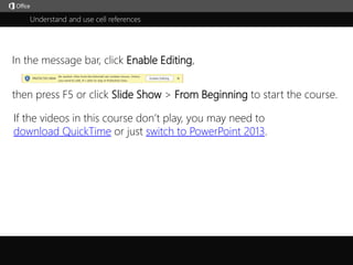
1. Understand and use cell references
j
then press F5 or click Slide Show > From Beginning to start the course.
In the message bar, click Enable Editing,
If the videos in this course don’t play, you may need to
download QuickTime or just switch to PowerPoint 2013.

2. 51 2 3 4
Course summary HelpUnderstand and use cell references Closed captions
1/2 videos
Summary Feedback HelpCell references Copy formulas
1:44 3:13
Press F5 to start, Esc to stop
51 2 3 4
In Excel 2013, one of the key things you’ll calculate are values in cells.Cells are the boxes you see in the grid of an Excel worksheet, like this one.Each cell is identified on a worksheet by its reference—the column letter and row number that intersect at the cell's location.This cell’s in column D and row 5, so it’s cell D5. The column always comes first in a cell reference.When you use cell references in a formula, in this case I’m adding cells A2 and B2,Excel calculates the answer using the numbers in the referenced cells.When I change the value in a cell, the formula calculates the new result automatically.Instead of typing each individual cell in a formula,you can reference multiple adjacent cells, called a range of cells.This range of cells is referred to as F2:G5. The first cell is F2 and the last cell is G5.You always start a formula with an equals sign. I’m using the SUM function in the formula to add this range
of cells.
And there we have the sum, or total, for the range of cells.Up next, copying formulas.

3. 51 2 3 4
Course summary HelpUnderstand and use cell references Closed captions
2/2 videos
Summary Feedback Help
Press F5 to start, Esc to stop
51 2 3 4
We just saw how to create a formula that adds two cells.Now let’s copy the formula down the column so it adds the other pairs of cells.The formula in C2 is A2 “+” B2. To copy it,1. Put the mouse pointer over the bottom right corner of the cell until it’s a black plus sign.2. Click and hold the left mouse button and drag the plus sign over the cells you want to fill.And the formula is copied into the other cells.But the formula wasn’t just copied.If it was just copied, all of the cells with the formula would have remained A2 “+” B2.And by looking at the results in each cell; that obviously hasn’t happened.Copying the formula from C2 to C3 increased the relative position of the formula by one rowbut didn’t change the column.The formula in C2 was A2 “+” B2.The formula in C3 is A3 “+” B3. The cell references in the formula increased by one row.The formulas in C4 and C5 updated similarly.This is called a relative cell reference and it’s the default for Excel.But you don’t always want cell references to change when you copy a formula.In this example, F2 is divided by E2. And we want the other numbers in column F to be divided by E2 as
well.
In other words, we want E2 to not change when the formula is copied.We can do that by making the reference absolute instead of relative.If we copy the formula like we did before, we get an error.For example, in G3 the copied formula is F3, which is 12, divided by E3, which is blank.Excel interprets a blank cell as a 0 and that’s a math error.To make E2 an absolute cell reference, I type a “$” before the E and a “$” before the 2 and press Enter.Now when we copy the formula we get the results we expect.When we look at the formula in G3, the first cell reference did update, as expected, but the E2 absolute cell
reference didn’t.
Neat!Now you’ve got a pretty good idea about what cell references are and how to use them.Of course, there’s always more to learn.So check out the course summary at the end, and best of all, explore Excel 2013 on your own.
Cell references Copy formulas
1:44 3:13

4. Help Course summary
Press F5 to start, Esc to stop
Course summary—Understand and use cell references
Summary Feedback Help
51 2 3 4
Cell references Copy formulas
1:44 3:13
Create a cell reference on the
same worksheet
1. Click the cell in which you want to enter the
formula.
2. In the formula bar, type = (equal sign).
3. Do one of the following:
• Reference one or more cells To create
a reference, select a cell or range of
cells on the same worksheet. Cell
references and the borders around the
corresponding cells are color-coded to
make it easier to work with them. You
can drag the border of the cell
selection to move the selection, or
drag the corner of the border to
expand the selection.
• Reference a defined name To create a
reference to a defined name, do one of
the following:
• Type the name.
• Press F3, select the name in the
Paste name box, and then click
OK.
4. Do one of the following:
• If you are creating a reference in a
single cell, press Enter.
• If you are creating a reference in an
array formula (such A1:G4), press
Ctrl+Shift+Enter.
The reference can be a single cell or
a range of cells, and the array
formula can be one that calculates
single or multiple results.
See also
• Create or change a cell reference
• Use cell references in a formula
• Create a reference to the same cell
range on multiple worksheets
• More training courses
• Office Compatibility Pack

5. Help Course summary
Press F5 to start, Esc to stop
Rating and comments
Thank you for viewing this course!
Please tell us what you think
Summary Feedback Help
51 2 3 4
Check out more courses
Cell references Copy formulas
1:44 3:13

6. Help Course summary
Press F5 to start, Esc to stop
Help
Summary Feedback Help
51 2 3 4
Using PowerPoint’s video controls
Going places
Stopping a course
If you download a course and the videos don’t play
get the PowerPoint Viewer. the QuickTime
player upgrade to PowerPoint 2013
Cell references Copy formulas
1:44 3:13