SlideShare una empresa de Scribd logo
1 de 9
FLUID MOTION IN THE POSTERIOR CHAMBER OF THE EYE.

1. INTRODUCTION.

The posterior chamber is a narrow chink behind the peripheral part of the iris of the
lens, and in front of the suspensory ligament of the lens and the ciliary processes. The
Posterior Chamber consists of small space directly posterior to the Iris but anterior to
the lens.


                            Figure 1: Human eye anatomy

The posterior chamber is filled with a watery fluid known as the aqueous humor, or
aqueous. Produced by a structure alongside the lens called the ciliary body, the
aqueous passes into the posterior chamber and then flows forward through the pupil
into the anterior chamber of the eye.

2. The equations of motion in cylindrical coordinates:

2.1   Assumption:

The main goal of this work is to find the velocity and pressure distribution profiles to
the fluid moving in vitreous chamber. To construct the model of the flow of aqueous


                                                                           Page 35 of 43
fluid in the vitreous (posterior) chamber of the eye let us consider following
assumptions:
     The aqueous fluid is Newtonian and incompressible fluid
     Asymmetric flow
     The height of the chamber is small compared to the radial length
     Neglect the flow in the region of the pupil
     Steady-state analysis
     Rigid iris


                         Figure 2: Simple model for the chamber

Consider equations of motion: the Equation of Continuity and Navier - Stokes Equation.
Here we work in the cylindrical coordinates. Hence we use the equations for the
cylindrical coordinates.

Where,
We consider geometry of the domain: Ri  r  Ro .


Let's   consider   cylindrical   coordinates    z, r ,     with     corresponding     velocity
components u z , u r , u  . According to the geometry of the system, there is no motion in
                                                                              u
φ direction and also the velocity is not a function of φ, i.e. u  0 and           0
                                                                              

Also, with the hypothesis of having incompressible fluid (  constant) and considering
the system in the steady-state (nothing is a function of time), the equation of motion
will be reduced to the followings:

                           u z 1 rur 
                                         0                     (1)
                            z r r


                                                                                    Page 36 of 43
This is called The Equation of Continuity. And The Navier Stokes Equations:


                  u r     u      P     1   rur    2 u r    
            ur         uz r        
                                            r r  r   z 2         
                                                                            (2)
                   r       z     r                              
                  u z     u      P     1   ru z    2 u z   
           ur          uz z        
                                            r r  r   z 2         
                                                                            (3)
                   r       z     z                              

2.2    Order of magnitude and simplification of the equation:

Characteristic dimensions:
   a) Characteristic velocity in the r-direction: U
   b) Characteristic dimension in the r-direction: L  Ri  Ro
   c) Characteristic dimension in the z-direction: H

If we denote the order of magnitude as O (.), we will have the followings:

                                            O(u r )  U
                                              u    U
                                            O r    
                                              r    L

Now from the continuity equation we have:

                                      u       1 rur   U
                                    O z   O             
                                      z       r r  L
                                                     UH
                                           O(u z ) 
                                                      L

Simplification of the equations in the r-direction:

                                               1 ru r    U
                                   1     O 
                                             r r r    L2 
                                                           
                                              2u  U
                                   2     O 2z   2
                                             z  H
                                                  

Since H << L we can neglect the expression (1) in comparison to expression (2). So
the equation in the r-direction would be

                                  u r      u r    P    2ur
                                 ur    uz           2
                                  r         z     r   z

                                                                             Page 37 of 43
Simplification of the equations in the z-direction:

                                            1    u z    UH 1
                                 1      O
                                            r r  r r    L . L2
                                                              
                                                          
                                             2 u z  UH 1
                                 2      O 2  
                                            z            .
                                                      L H2


Again since H << L we can neglect the expression 1 in comparison to expression 2 .So
the equation in the z-direction reads

                                        u z     u      P     2u
                                  ur         uz z         2z
                                         r       z     z    z

Scaling and comparing the equations in the r and z direction

Knowing the order of magnitude of the expressions in r and z direction, we make the
equations dimensionless as follows:


                           U2    * u r
                                       *
                                              u r 
                                                 *
                                                     P P *    U  2u *
                                u r *  u * *    o . *   2 *2r
                                 r          z     L r     H z
                                            z
                           L                      
                           U2    * u *      u *  P P *     U  2u *
                                u r *  u * *    o . *   2 *2z
                                 r
                                       z         z

                                              z     L z      H z
                                            z
                           L                      

             H
Where,        1 , P  Po P * and Po will be specified later.
             L

Then we have,


                           UH  * u r
                                     *
                                          * u r 
                                               *
                                                    H 2 Po P *  2 u r
                                                                      *
                             ur      uz *          .    
                              r *
                                           z    UL r * z *2
                             UH  * u *     u *   H 2 Po P *   2u *
                       2       ur *  u * *   
                                       z        z
                                                           . *   *2z
                                r         z      UL z     z
                                           z
                                                 

According to the above equations, we can find the proper scaling for Po by balancing
with the viscous terms. This leads to
                                                       UL
                                                Po 
                                                       H2


                                                                           Page 38 of 43
Now, if we multiply the equation of motion in the z-direction by  , you can neglect the
terms with  2 &  3 and we will end up with
                                               P *
                                                    0
                                               z *

This suggests that P is not a function of z. Therefore, pressure is just a function of r,
i.e. P  f r 

2.3 Further simplification in r-direction:

By neglecting the nonlinear part of the equation of motion in the r-direction and here
our problem is a type of lubrication theory, so we have:

                                                     UH
                                              Re 
                                                      
Therefore we can write:

                                       u r
                                           *
                                                   u r 
                                                      *
                                                           P *  2 u *
                           Re  u r*
                                             u * *   . *  *2r
                                        r *       z     r   z
                                                 z
                                                       

Now if  .Re  1 , then we can neglect the non-linear part in the equation of motion.
Since the Reynolds number for the aqueous humor is approximately 10 3 [1], then the
above condition holds. Therefore, we can reduce the equation of motion in the r-
direction to the following:

                                             P     2ur
                                                                                      (1)
                                             r     z 2

Integrating the equation (1) with respect to z, we will reach

                                            1  P  2
                                    ur         z  c1 z  c 2
                                           2  r 

We can find the constants c1 and c 2 , using the no-slip conditions


                                    u r ( z  0)  u r ( z  H )  0
                                             H  p 
                                    c1         
                                             2  r 
                                    c2  0


                                                                              Page 39 of 43
Substituting the constants in the equation of motion we have


                                           H  P  z     z
                                                           2

                          u r ( z, r )                                          (2)
                                           2  r  H 
                                                            H
                                                              

Here for simplicity we consider the height H to be constant in our calculation.
For H  hr  , the calculation process is similar.
Now, the only undetermined term in the velocity profile is the pressure distribution
which will be calculated as follows:

2.4   Pressure distribution:

Integrating the continuity equation with respect to z, from 0 to H, we will have
                                      u z        1 ru r 
                                    H           H

                                     z
                                    0
                                           dz  
                                                0
                                                  r r
                                                            dz  0

                                                             1 ru r 
                                                          H
                               uz          uz                       dz  0
                                    zH          z 0
                                                           0
                                                             r r


Using the no-slip conditions
                                          uz   zH
                                                         uz   z 0
                                                                      0


We will end up having


                                             1 ru r 
                                           H

                                            r r dz  0
                                           0

                                          1               
                                                   H
                                                r  u r dz   0
                                               
                                          r r  0          
                                                            

Since r  0
                                                         
                                                  H
                                               r  u r dz   0
                                           r  0
                                              
                                                           
                                                           
                                                  H
                                                 r  ur dz  c
                                                  0

Where, c is a constant.


                                                                                Page 40 of 43
Since r  0
                                              H
                                                          c
                                                u dz  r
                                               0
                                                    r


Substituting u r into the equation and computing the integral, we will get


                                              H 3 P   c
                                                 ( )                                   (3)
                                              12 r   r

To find the constant c, we integrate the equation as follows:

                                                              H3
                                   Let's call, A  
                                                              12
                                          P0             R0
                                                             dr
                                      A  dp  c 
                                          Pi              Ri
                                                             r
                                                              R0
                                    A( P0  Pi )  c(ln          )
                                                              Ri
                                                   A( P0  Pi )
                                      c
                                                        R
                                                     ln 0
                                                         Ri


Calculating the indefinite integral of equation (3), we get the pressure distribution:

                                               P0  Pi
                                  P(r )               ln r  k
                                                  R0
                                               ln( )
                                                  Ri


To find the constant k, we know that P(r  Ri )  Pi and therefore:


                                                   P0  P
                                  kP
                                    i
                                                         i
                                                           ln( Ri )
                                                      R0
                                                   ln( )
                                                      Ri
                                          P0  Pi    r
                                P(r )            ln( )  Pi                             (4)
                                             R       Ri
                                          ln( 0 )
                                             Ri


                                                                              Page 41 of 43
2.5   Velocity Profile:

Substituting the derivative of the pressure distribution in equation (2) for velocity
profile, we get
                                       H 2 1 P0  Pi z 2 z
                      ur ( z , r )                 [( )  ]                           (5)
                                       2 r ln( R0 ) H    H
                                                Ri


Here one can make the calculation more accurate by considering the height of the
posterior chamber to be a function of r rather than being constant. In this case, based
on the model in Figure 1, one may substitute H in equation (3) with h(r ) which has the
following equation:
                                             h(r )  m.r  k
Where,
                                              k  h0  R0 m
                                                   hi  h0                             (6)
                                              m
                                                   Ri  R 0


Then, following similar procedure one can get the pressure distribution and velocity
profile.

3. CONCLUSION:

Pressure distribution: The highest pressure is at the radius Ri where P(r  Ri )  Pi . As
we move along the r-direction toward the pupil, the pressure drops logarithmically
  P  Pi    r
by 0     ln( ) . If we increase P0  Pi (keeping the values Ri and Ro constant), we
     R      Ri
   ln 0
     Ri
will have a larger pressure drop in the posterior chamber.

Knowing the pressure distribution is very important in studying the glaucoma. In the
severe glaucoma (closed-angle glaucoma), eye pressure builds up rapidly when the
drainage area (trabecular meshwork) suddenly becomes blocked, in this case the high
amount of pressure in the posterior chamber results in increase of the fluid pressure
within the inner eye , which can damage the optic nerve and lead to vision loss.


                                                                             Page 42 of 43
3.1    Velocity profile:

The aqueous humor has the following characteristics

       Density   1000kg.m 3
       Viscosity   7.5  10 4 kg.m 1 .s 1
       Characteristic length scale H  2  10 6 m

From the equation (5) for the velocity profile, one can notice that the highest velocity is
                  H
at r  Ro and z  , i.e. exactly at the entrance to the pupil. Based on [1], the
                   2
maximum velocity of the aqueous humor is 1.01m.s 1 , which is about 3rd orders bigger
than the velocity in the anterior and posterior chambers.

4. REFERENCE:

[1] Jeffrey J. Heys, Victor H. Barocas and Michael J. Taravella; Modeling Passive
    Mechanical Interaction between Aqueous Humor and Iris, Journal of
    Biomechanical Engineering, Dec. 2001, vol. 123(6), p.p. 540-7.
[2] Repetto, R., Tatone, A., Testa, A. and Colangeli, E. 2011. Traction on the Retina
    Induced by Saccadic Eye Movements in the Presence of Posterior Vitreous
    Detachment. Biomech. Model. Mechanobiol., vol. 10, pp. 191-202,
    doi:10.1007/s10237-010-0226-6.
[3] Repetto, R., Siggers, J. H. and Stocchino, A. 2010. Mathematical model of flow in
    the vitreous humor induced by saccadic eye rotations: effect of geometry.
    Biomech. Model. Mechanobiol., vol. 9, pp. 65-76.
[4] Stocchino, A., Repetto, R. and Siggers, J. H. Mixing processes in the vitreous
    chamber induced by eye rotations. 2010. Phys. Med. Biol, vol. 55, pp. 453-467.
[5] R. Byron Bird, Warren E. Stewart and Edwin N. Lightfoot. Transport Phenomena.
    2nd edition.


                                                                              Page 43 of 43

Más contenido relacionado

La actualidad más candente

refractive surgeries
refractive surgeriesrefractive surgeries
refractive surgeries
nehapathak88
 
Proptosis investigation & management.rdh
Proptosis investigation & management.rdhProptosis investigation & management.rdh
Proptosis investigation & management.rdh
radhe4827
 

La actualidad más candente (20)

41 principles retinal detachment surgery
41 principles retinal detachment surgery41 principles retinal detachment surgery
41 principles retinal detachment surgery
 
Polypoidal choroidal vasculopathy
Polypoidal choroidal vasculopathyPolypoidal choroidal vasculopathy
Polypoidal choroidal vasculopathy
 
Vitrectomy Principles
Vitrectomy PrinciplesVitrectomy Principles
Vitrectomy Principles
 
Retina
RetinaRetina
Retina
 
refractive surgeries
refractive surgeriesrefractive surgeries
refractive surgeries
 
The ocular presentation of systemic diseases
The ocular presentation of systemic diseasesThe ocular presentation of systemic diseases
The ocular presentation of systemic diseases
 
Optic nerve head evaluation
Optic nerve head evaluationOptic nerve head evaluation
Optic nerve head evaluation
 
Proptosis investigation & management.rdh
Proptosis investigation & management.rdhProptosis investigation & management.rdh
Proptosis investigation & management.rdh
 
Retina drwaing
Retina drwaingRetina drwaing
Retina drwaing
 
Refractive surgery basics, LASIK
Refractive surgery basics, LASIKRefractive surgery basics, LASIK
Refractive surgery basics, LASIK
 
OCT – Introduction and Macular disorders
OCT – Introduction and Macular disordersOCT – Introduction and Macular disorders
OCT – Introduction and Macular disorders
 
Proptosis
ProptosisProptosis
Proptosis
 
Aqueous humor dynamics
Aqueous humor dynamics Aqueous humor dynamics
Aqueous humor dynamics
 
anatomy and physiology of the lens
anatomy and physiology of the lensanatomy and physiology of the lens
anatomy and physiology of the lens
 
Pupil And its Abnormalities
Pupil And its AbnormalitiesPupil And its Abnormalities
Pupil And its Abnormalities
 
Scleral fixation technique
Scleral fixation techniqueScleral fixation technique
Scleral fixation technique
 
Retina preliminary
Retina  preliminaryRetina  preliminary
Retina preliminary
 
Functional vision loss - Differentiating functional vision loss from malinger...
Functional vision loss - Differentiating functional vision loss from malinger...Functional vision loss - Differentiating functional vision loss from malinger...
Functional vision loss - Differentiating functional vision loss from malinger...
 
Prescription of glasses in children
Prescription of glasses in childrenPrescription of glasses in children
Prescription of glasses in children
 
Vitreous humour in our eyeballs
Vitreous humour in our eyeballs Vitreous humour in our eyeballs
Vitreous humour in our eyeballs
 

Destacado

Engineering Drawing
Engineering DrawingEngineering Drawing
Engineering Drawing
Lai Chun Tat
 
Study of wind effect on building with hexagonal cross section
Study of wind effect on building with hexagonal cross sectionStudy of wind effect on building with hexagonal cross section
Study of wind effect on building with hexagonal cross section
Dr. Bhuiyan S. M. Ebna Hai
 
AR101 -POLIBRIGED ( PERTOLONGAN CEMAS)
AR101 -POLIBRIGED ( PERTOLONGAN CEMAS)AR101 -POLIBRIGED ( PERTOLONGAN CEMAS)
AR101 -POLIBRIGED ( PERTOLONGAN CEMAS)
mokhtar
 
Engineering Drawing: Chapter 12 working drawing
Engineering Drawing: Chapter 12 working drawingEngineering Drawing: Chapter 12 working drawing
Engineering Drawing: Chapter 12 working drawing
mokhtar
 
Eg unit iii-projection_of_points
Eg unit iii-projection_of_pointsEg unit iii-projection_of_points
Eg unit iii-projection_of_points
justinjacob1993
 

Destacado (20)

Engineering Drawing
Engineering DrawingEngineering Drawing
Engineering Drawing
 
Engineering Drawing
Engineering DrawingEngineering Drawing
Engineering Drawing
 
Dimensioning rules in engineering drawing
Dimensioning rules in engineering drawingDimensioning rules in engineering drawing
Dimensioning rules in engineering drawing
 
A simple model of the liver microcirculation
A simple model of the liver microcirculationA simple model of the liver microcirculation
A simple model of the liver microcirculation
 
Study of wind effect on building with hexagonal cross section
Study of wind effect on building with hexagonal cross sectionStudy of wind effect on building with hexagonal cross section
Study of wind effect on building with hexagonal cross section
 
Dynamic behavior of catalytic converters
Dynamic behavior of catalytic convertersDynamic behavior of catalytic converters
Dynamic behavior of catalytic converters
 
Design Analysis Of Uav (Unmanned Air Vehicle) Using NACA 0012 Aerofoil Profile
Design Analysis Of Uav (Unmanned Air Vehicle) Using NACA 0012 Aerofoil ProfileDesign Analysis Of Uav (Unmanned Air Vehicle) Using NACA 0012 Aerofoil Profile
Design Analysis Of Uav (Unmanned Air Vehicle) Using NACA 0012 Aerofoil Profile
 
Introduction to Engineering drawing and Graphics
Introduction to Engineering drawing and GraphicsIntroduction to Engineering drawing and Graphics
Introduction to Engineering drawing and Graphics
 
AR101 -POLIBRIGED ( PERTOLONGAN CEMAS)
AR101 -POLIBRIGED ( PERTOLONGAN CEMAS)AR101 -POLIBRIGED ( PERTOLONGAN CEMAS)
AR101 -POLIBRIGED ( PERTOLONGAN CEMAS)
 
Engineering Drawing: Chapter 12 working drawing
Engineering Drawing: Chapter 12 working drawingEngineering Drawing: Chapter 12 working drawing
Engineering Drawing: Chapter 12 working drawing
 
TECHNICAL DRAWING
TECHNICAL DRAWINGTECHNICAL DRAWING
TECHNICAL DRAWING
 
BE sem 1 Engineering Graphics(E.G.) full course ppt
BE sem 1 Engineering Graphics(E.G.) full course pptBE sem 1 Engineering Graphics(E.G.) full course ppt
BE sem 1 Engineering Graphics(E.G.) full course ppt
 
Basic Mechanical Engineering drawing
Basic Mechanical Engineering drawingBasic Mechanical Engineering drawing
Basic Mechanical Engineering drawing
 
Study of Aerodynamics of a Cricket Ball
Study of Aerodynamics of a Cricket BallStudy of Aerodynamics of a Cricket Ball
Study of Aerodynamics of a Cricket Ball
 
Descriptive geometry
Descriptive  geometryDescriptive  geometry
Descriptive geometry
 
Instruction course-Secondary posterior chamber IOL (PC IOL) Implantation-made...
Instruction course-Secondary posterior chamber IOL (PC IOL) Implantation-made...Instruction course-Secondary posterior chamber IOL (PC IOL) Implantation-made...
Instruction course-Secondary posterior chamber IOL (PC IOL) Implantation-made...
 
angle of projections
angle of projectionsangle of projections
angle of projections
 
Anatomy of the eye
Anatomy of the eyeAnatomy of the eye
Anatomy of the eye
 
Modelling and Analysis Laboratory Manual
Modelling and Analysis Laboratory ManualModelling and Analysis Laboratory Manual
Modelling and Analysis Laboratory Manual
 
Eg unit iii-projection_of_points
Eg unit iii-projection_of_pointsEg unit iii-projection_of_points
Eg unit iii-projection_of_points
 

Similar a Fluid motion in the posterior chamber of the eye

Speech waves in tube and filters
Speech waves in tube and filtersSpeech waves in tube and filters
Speech waves in tube and filters
Nikolay Karpov
 
IJCER (www.ijceronline.com) International Journal of computational Engineerin...
IJCER (www.ijceronline.com) International Journal of computational Engineerin...IJCER (www.ijceronline.com) International Journal of computational Engineerin...
IJCER (www.ijceronline.com) International Journal of computational Engineerin...
ijceronline
 
The shortest distance between skew lines
The shortest distance between skew linesThe shortest distance between skew lines
The shortest distance between skew lines
Tarun Gehlot
 
IJCER (www.ijceronline.com) International Journal of computational Engineerin...
IJCER (www.ijceronline.com) International Journal of computational Engineerin...IJCER (www.ijceronline.com) International Journal of computational Engineerin...
IJCER (www.ijceronline.com) International Journal of computational Engineerin...
ijceronline
 
DIFFERENT ATOMIC MODELS
DIFFERENT ATOMIC MODELSDIFFERENT ATOMIC MODELS
DIFFERENT ATOMIC MODELS
Shahn Tee
 

Similar a Fluid motion in the posterior chamber of the eye (15)

Speech waves in tube and filters
Speech waves in tube and filtersSpeech waves in tube and filters
Speech waves in tube and filters
 
International Journal of Engineering Inventions (IJEI)
International Journal of Engineering Inventions (IJEI)International Journal of Engineering Inventions (IJEI)
International Journal of Engineering Inventions (IJEI)
 
Shell Momentum Balances in heat transfer
Shell Momentum Balances in heat transferShell Momentum Balances in heat transfer
Shell Momentum Balances in heat transfer
 
07
0707
07
 
IJCER (www.ijceronline.com) International Journal of computational Engineerin...
IJCER (www.ijceronline.com) International Journal of computational Engineerin...IJCER (www.ijceronline.com) International Journal of computational Engineerin...
IJCER (www.ijceronline.com) International Journal of computational Engineerin...
 
The shortest distance between skew lines
The shortest distance between skew linesThe shortest distance between skew lines
The shortest distance between skew lines
 
Orthogonal Decomp. Thm
Orthogonal Decomp. ThmOrthogonal Decomp. Thm
Orthogonal Decomp. Thm
 
lecture33.pptx
lecture33.pptxlecture33.pptx
lecture33.pptx
 
boundary_layers_History.ppt
boundary_layers_History.pptboundary_layers_History.ppt
boundary_layers_History.ppt
 
GFD07_boundary_layers_24629.ppt
GFD07_boundary_layers_24629.pptGFD07_boundary_layers_24629.ppt
GFD07_boundary_layers_24629.ppt
 
Decay Property for Solutions to Plate Type Equations with Variable Coefficients
Decay Property for Solutions to Plate Type Equations with Variable CoefficientsDecay Property for Solutions to Plate Type Equations with Variable Coefficients
Decay Property for Solutions to Plate Type Equations with Variable Coefficients
 
IJCER (www.ijceronline.com) International Journal of computational Engineerin...
IJCER (www.ijceronline.com) International Journal of computational Engineerin...IJCER (www.ijceronline.com) International Journal of computational Engineerin...
IJCER (www.ijceronline.com) International Journal of computational Engineerin...
 
Talk spinoam photon
Talk spinoam photonTalk spinoam photon
Talk spinoam photon
 
DIFFERENT ATOMIC MODELS
DIFFERENT ATOMIC MODELSDIFFERENT ATOMIC MODELS
DIFFERENT ATOMIC MODELS
 
character table in vibrational spectroscopy
character table in vibrational spectroscopycharacter table in vibrational spectroscopy
character table in vibrational spectroscopy
 

Último

Spellings Wk 3 English CAPS CARES Please Practise
Spellings Wk 3 English CAPS CARES Please PractiseSpellings Wk 3 English CAPS CARES Please Practise
Spellings Wk 3 English CAPS CARES Please Practise
AnaAcapella
 
Jual Obat Aborsi Hongkong ( Asli No.1 ) 085657271886 Obat Penggugur Kandungan...
Jual Obat Aborsi Hongkong ( Asli No.1 ) 085657271886 Obat Penggugur Kandungan...Jual Obat Aborsi Hongkong ( Asli No.1 ) 085657271886 Obat Penggugur Kandungan...
Jual Obat Aborsi Hongkong ( Asli No.1 ) 085657271886 Obat Penggugur Kandungan...
ZurliaSoop
 
The basics of sentences session 3pptx.pptx
The basics of sentences session 3pptx.pptxThe basics of sentences session 3pptx.pptx
The basics of sentences session 3pptx.pptx
heathfieldcps1
 

Último (20)

Understanding Accommodations and Modifications
Understanding  Accommodations and ModificationsUnderstanding  Accommodations and Modifications
Understanding Accommodations and Modifications
 
Spellings Wk 3 English CAPS CARES Please Practise
Spellings Wk 3 English CAPS CARES Please PractiseSpellings Wk 3 English CAPS CARES Please Practise
Spellings Wk 3 English CAPS CARES Please Practise
 
Mixin Classes in Odoo 17 How to Extend Models Using Mixin Classes
Mixin Classes in Odoo 17  How to Extend Models Using Mixin ClassesMixin Classes in Odoo 17  How to Extend Models Using Mixin Classes
Mixin Classes in Odoo 17 How to Extend Models Using Mixin Classes
 
Sociology 101 Demonstration of Learning Exhibit
Sociology 101 Demonstration of Learning ExhibitSociology 101 Demonstration of Learning Exhibit
Sociology 101 Demonstration of Learning Exhibit
 
This PowerPoint helps students to consider the concept of infinity.
This PowerPoint helps students to consider the concept of infinity.This PowerPoint helps students to consider the concept of infinity.
This PowerPoint helps students to consider the concept of infinity.
 
Unit-IV- Pharma. Marketing Channels.pptx
Unit-IV- Pharma. Marketing Channels.pptxUnit-IV- Pharma. Marketing Channels.pptx
Unit-IV- Pharma. Marketing Channels.pptx
 
2024-NATIONAL-LEARNING-CAMP-AND-OTHER.pptx
2024-NATIONAL-LEARNING-CAMP-AND-OTHER.pptx2024-NATIONAL-LEARNING-CAMP-AND-OTHER.pptx
2024-NATIONAL-LEARNING-CAMP-AND-OTHER.pptx
 
Making communications land - Are they received and understood as intended? we...
Making communications land - Are they received and understood as intended? we...Making communications land - Are they received and understood as intended? we...
Making communications land - Are they received and understood as intended? we...
 
Unit-V; Pricing (Pharma Marketing Management).pptx
Unit-V; Pricing (Pharma Marketing Management).pptxUnit-V; Pricing (Pharma Marketing Management).pptx
Unit-V; Pricing (Pharma Marketing Management).pptx
 
How to Give a Domain for a Field in Odoo 17
How to Give a Domain for a Field in Odoo 17How to Give a Domain for a Field in Odoo 17
How to Give a Domain for a Field in Odoo 17
 
TỔNG ÔN TẬP THI VÀO LỚP 10 MÔN TIẾNG ANH NĂM HỌC 2023 - 2024 CÓ ĐÁP ÁN (NGỮ Â...
TỔNG ÔN TẬP THI VÀO LỚP 10 MÔN TIẾNG ANH NĂM HỌC 2023 - 2024 CÓ ĐÁP ÁN (NGỮ Â...TỔNG ÔN TẬP THI VÀO LỚP 10 MÔN TIẾNG ANH NĂM HỌC 2023 - 2024 CÓ ĐÁP ÁN (NGỮ Â...
TỔNG ÔN TẬP THI VÀO LỚP 10 MÔN TIẾNG ANH NĂM HỌC 2023 - 2024 CÓ ĐÁP ÁN (NGỮ Â...
 
psychiatric nursing HISTORY COLLECTION .docx
psychiatric  nursing HISTORY  COLLECTION  .docxpsychiatric  nursing HISTORY  COLLECTION  .docx
psychiatric nursing HISTORY COLLECTION .docx
 
How to Create and Manage Wizard in Odoo 17
How to Create and Manage Wizard in Odoo 17How to Create and Manage Wizard in Odoo 17
How to Create and Manage Wizard in Odoo 17
 
Food safety_Challenges food safety laboratories_.pdf
Food safety_Challenges food safety laboratories_.pdfFood safety_Challenges food safety laboratories_.pdf
Food safety_Challenges food safety laboratories_.pdf
 
Kodo Millet PPT made by Ghanshyam bairwa college of Agriculture kumher bhara...
Kodo Millet  PPT made by Ghanshyam bairwa college of Agriculture kumher bhara...Kodo Millet  PPT made by Ghanshyam bairwa college of Agriculture kumher bhara...
Kodo Millet PPT made by Ghanshyam bairwa college of Agriculture kumher bhara...
 
SKILL OF INTRODUCING THE LESSON MICRO SKILLS.pptx
SKILL OF INTRODUCING THE LESSON MICRO SKILLS.pptxSKILL OF INTRODUCING THE LESSON MICRO SKILLS.pptx
SKILL OF INTRODUCING THE LESSON MICRO SKILLS.pptx
 
Jual Obat Aborsi Hongkong ( Asli No.1 ) 085657271886 Obat Penggugur Kandungan...
Jual Obat Aborsi Hongkong ( Asli No.1 ) 085657271886 Obat Penggugur Kandungan...Jual Obat Aborsi Hongkong ( Asli No.1 ) 085657271886 Obat Penggugur Kandungan...
Jual Obat Aborsi Hongkong ( Asli No.1 ) 085657271886 Obat Penggugur Kandungan...
 
The basics of sentences session 3pptx.pptx
The basics of sentences session 3pptx.pptxThe basics of sentences session 3pptx.pptx
The basics of sentences session 3pptx.pptx
 
SOC 101 Demonstration of Learning Presentation
SOC 101 Demonstration of Learning PresentationSOC 101 Demonstration of Learning Presentation
SOC 101 Demonstration of Learning Presentation
 
ComPTIA Overview | Comptia Security+ Book SY0-701
ComPTIA Overview | Comptia Security+ Book SY0-701ComPTIA Overview | Comptia Security+ Book SY0-701
ComPTIA Overview | Comptia Security+ Book SY0-701
 

Fluid motion in the posterior chamber of the eye

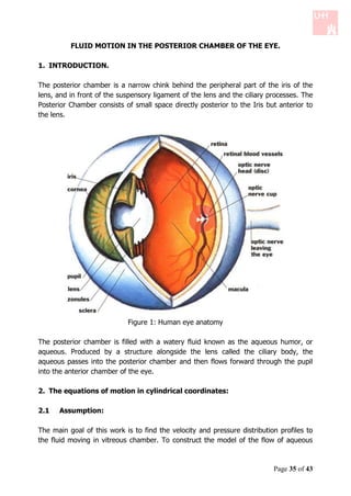
  • 1. FLUID MOTION IN THE POSTERIOR CHAMBER OF THE EYE. 1. INTRODUCTION. The posterior chamber is a narrow chink behind the peripheral part of the iris of the lens, and in front of the suspensory ligament of the lens and the ciliary processes. The Posterior Chamber consists of small space directly posterior to the Iris but anterior to the lens. Figure 1: Human eye anatomy The posterior chamber is filled with a watery fluid known as the aqueous humor, or aqueous. Produced by a structure alongside the lens called the ciliary body, the aqueous passes into the posterior chamber and then flows forward through the pupil into the anterior chamber of the eye. 2. The equations of motion in cylindrical coordinates: 2.1 Assumption: The main goal of this work is to find the velocity and pressure distribution profiles to the fluid moving in vitreous chamber. To construct the model of the flow of aqueous Page 35 of 43
  • 2. fluid in the vitreous (posterior) chamber of the eye let us consider following assumptions:  The aqueous fluid is Newtonian and incompressible fluid  Asymmetric flow  The height of the chamber is small compared to the radial length  Neglect the flow in the region of the pupil  Steady-state analysis  Rigid iris Figure 2: Simple model for the chamber Consider equations of motion: the Equation of Continuity and Navier - Stokes Equation. Here we work in the cylindrical coordinates. Hence we use the equations for the cylindrical coordinates. Where, We consider geometry of the domain: Ri  r  Ro . Let's consider cylindrical coordinates z, r ,   with corresponding velocity components u z , u r , u  . According to the geometry of the system, there is no motion in u φ direction and also the velocity is not a function of φ, i.e. u  0 and 0  Also, with the hypothesis of having incompressible fluid (  constant) and considering the system in the steady-state (nothing is a function of time), the equation of motion will be reduced to the followings: u z 1 rur   0 (1) z r r Page 36 of 43
  • 3. This is called The Equation of Continuity. And The Navier Stokes Equations:  u r u  P  1   rur    2 u r   ur  uz r       r r  r   z 2   (2)  r z  r      u z u  P  1   ru z    2 u z   ur  uz z       r r  r   z 2   (3)  r z  z     2.2 Order of magnitude and simplification of the equation: Characteristic dimensions: a) Characteristic velocity in the r-direction: U b) Characteristic dimension in the r-direction: L  Ri  Ro c) Characteristic dimension in the z-direction: H If we denote the order of magnitude as O (.), we will have the followings: O(u r )  U  u  U O r   r  L Now from the continuity equation we have:  u   1 rur   U O z   O   z   r r  L UH O(u z )  L Simplification of the equations in the r-direction:    1 ru r    U 1 O   r r r    L2       2u  U 2 O 2z   2  z  H   Since H << L we can neglect the expression (1) in comparison to expression (2). So the equation in the r-direction would be  u r u r  P  2ur  ur  uz   2  r z  r z Page 37 of 43
  • 4. Simplification of the equations in the z-direction:  1    u z    UH 1 1 O  r r  r r    L . L2       2 u z  UH 1 2 O 2    z  .   L H2 Again since H << L we can neglect the expression 1 in comparison to expression 2 .So the equation in the z-direction reads  u z u  P  2u  ur  uz z      2z  r z  z z Scaling and comparing the equations in the r and z direction Knowing the order of magnitude of the expressions in r and z direction, we make the equations dimensionless as follows: U2  * u r * u r  * P P * U  2u *   u r *  u * *    o . *   2 *2r  r z  L r H z z L   U2  * u * u *  P P * U  2u *   u r *  u * *    o . *   2 *2z  r z z z  L z H z z L   H Where,    1 , P  Po P * and Po will be specified later. L Then we have, UH  * u r * * u r  * H 2 Po P *  2 u r *   ur  uz *    .    r *  z   UL r * z *2 UH  * u * u *  H 2 Po P *  2u *  2  ur *  u * *    z z . *   *2z   r z   UL z z z   According to the above equations, we can find the proper scaling for Po by balancing with the viscous terms. This leads to UL Po  H2 Page 38 of 43
  • 5. Now, if we multiply the equation of motion in the z-direction by  , you can neglect the terms with  2 &  3 and we will end up with P * 0 z * This suggests that P is not a function of z. Therefore, pressure is just a function of r, i.e. P  f r  2.3 Further simplification in r-direction: By neglecting the nonlinear part of the equation of motion in the r-direction and here our problem is a type of lubrication theory, so we have: UH Re   Therefore we can write:  u r * u r  * P *  2 u * Re  u r*   u * *   . *  *2r r * z  r z z   Now if  .Re  1 , then we can neglect the non-linear part in the equation of motion. Since the Reynolds number for the aqueous humor is approximately 10 3 [1], then the above condition holds. Therefore, we can reduce the equation of motion in the r- direction to the following: P  2ur  (1) r z 2 Integrating the equation (1) with respect to z, we will reach 1  P  2 ur    z  c1 z  c 2 2  r  We can find the constants c1 and c 2 , using the no-slip conditions u r ( z  0)  u r ( z  H )  0 H  p  c1     2  r  c2  0 Page 39 of 43
  • 6. Substituting the constants in the equation of motion we have H  P  z  z 2 u r ( z, r )        (2) 2  r  H   H  Here for simplicity we consider the height H to be constant in our calculation. For H  hr  , the calculation process is similar. Now, the only undetermined term in the velocity profile is the pressure distribution which will be calculated as follows: 2.4 Pressure distribution: Integrating the continuity equation with respect to z, from 0 to H, we will have u z 1 ru r  H H  z 0 dz   0 r r dz  0 1 ru r  H uz  uz  dz  0 zH z 0 0 r r Using the no-slip conditions uz zH  uz z 0 0 We will end up having 1 ru r  H  r r dz  0 0 1    H  r  u r dz   0  r r  0   Since r  0    H  r  u r dz   0 r  0    H r  ur dz  c 0 Where, c is a constant. Page 40 of 43
  • 7. Since r  0 H c  u dz  r 0 r Substituting u r into the equation and computing the integral, we will get H 3 P c  ( ) (3) 12 r r To find the constant c, we integrate the equation as follows: H3 Let's call, A   12 P0 R0 dr A  dp  c  Pi Ri r R0 A( P0  Pi )  c(ln ) Ri A( P0  Pi ) c R ln 0 Ri Calculating the indefinite integral of equation (3), we get the pressure distribution: P0  Pi P(r )  ln r  k R0 ln( ) Ri To find the constant k, we know that P(r  Ri )  Pi and therefore: P0  P kP i i ln( Ri ) R0 ln( ) Ri P0  Pi r P(r )  ln( )  Pi (4) R Ri ln( 0 ) Ri Page 41 of 43
  • 8. 2.5 Velocity Profile: Substituting the derivative of the pressure distribution in equation (2) for velocity profile, we get H 2 1 P0  Pi z 2 z ur ( z , r )  [( )  ] (5) 2 r ln( R0 ) H H Ri Here one can make the calculation more accurate by considering the height of the posterior chamber to be a function of r rather than being constant. In this case, based on the model in Figure 1, one may substitute H in equation (3) with h(r ) which has the following equation: h(r )  m.r  k Where, k  h0  R0 m hi  h0 (6) m Ri  R 0 Then, following similar procedure one can get the pressure distribution and velocity profile. 3. CONCLUSION: Pressure distribution: The highest pressure is at the radius Ri where P(r  Ri )  Pi . As we move along the r-direction toward the pupil, the pressure drops logarithmically P  Pi r by 0 ln( ) . If we increase P0  Pi (keeping the values Ri and Ro constant), we R Ri ln 0 Ri will have a larger pressure drop in the posterior chamber. Knowing the pressure distribution is very important in studying the glaucoma. In the severe glaucoma (closed-angle glaucoma), eye pressure builds up rapidly when the drainage area (trabecular meshwork) suddenly becomes blocked, in this case the high amount of pressure in the posterior chamber results in increase of the fluid pressure within the inner eye , which can damage the optic nerve and lead to vision loss. Page 42 of 43
  • 9. 3.1 Velocity profile: The aqueous humor has the following characteristics Density   1000kg.m 3 Viscosity   7.5  10 4 kg.m 1 .s 1 Characteristic length scale H  2  10 6 m From the equation (5) for the velocity profile, one can notice that the highest velocity is H at r  Ro and z  , i.e. exactly at the entrance to the pupil. Based on [1], the 2 maximum velocity of the aqueous humor is 1.01m.s 1 , which is about 3rd orders bigger than the velocity in the anterior and posterior chambers. 4. REFERENCE: [1] Jeffrey J. Heys, Victor H. Barocas and Michael J. Taravella; Modeling Passive Mechanical Interaction between Aqueous Humor and Iris, Journal of Biomechanical Engineering, Dec. 2001, vol. 123(6), p.p. 540-7. [2] Repetto, R., Tatone, A., Testa, A. and Colangeli, E. 2011. Traction on the Retina Induced by Saccadic Eye Movements in the Presence of Posterior Vitreous Detachment. Biomech. Model. Mechanobiol., vol. 10, pp. 191-202, doi:10.1007/s10237-010-0226-6. [3] Repetto, R., Siggers, J. H. and Stocchino, A. 2010. Mathematical model of flow in the vitreous humor induced by saccadic eye rotations: effect of geometry. Biomech. Model. Mechanobiol., vol. 9, pp. 65-76. [4] Stocchino, A., Repetto, R. and Siggers, J. H. Mixing processes in the vitreous chamber induced by eye rotations. 2010. Phys. Med. Biol, vol. 55, pp. 453-467. [5] R. Byron Bird, Warren E. Stewart and Edwin N. Lightfoot. Transport Phenomena. 2nd edition. Page 43 of 43