learn about cp , cpk , pp , ppk and also learn how to build in excel

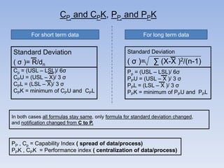
1. CP, and CPK, PP, and PPK
For short term data
For long term data
Standard Deviation
( σ )= R/dn
Standard Deviation
Cp = (USL – LSL)/ 6σ
CPU = (USL – X)/ 3 σ
CPL = (LSL – X)/ 3 σ
CPK = minimum of CPU and CPL
Pp = (USL – LSL)/ 6σ
PPU = (USL – X )/ 3 σ
PPL = (LSL – X )/ 3 σ
PPK = minimum of PPU and PPL
( σ )=
∑ (X-X )2/(n-1)
In both cases all formulas stay same, only formula for standard deviation changed,
and notification changed from C to P.
PP , Cp = Capability Index ( spread of data/process)
PPK , CPK = Performance index ( centralization of data/process)

2. All of 1st understand CP and CPK Graphically
Upper specified limit
CP
LSL
14
12
10
8
6
4
2
0
CPU
Center line
Axis Title
CPL
USL
Lower specified limit
Desired location of
data, centralized.
good Cp K
1 2 3 4 5 6 7 8 9 1011121314151617181920
0 1 2 3 4 5 6 7 8 9 10111213141516171819
Axis Title
All Data looks to be inside of this yellow curve, mean good spread of data.
Mean good CP.
But all data is not centralized, it is towards LSL , So we can get high number of
rejections, mean – CPK is not good.

3. To study, Cp, CpK, Pp , PpK you must know HISTOGRAM .
If you don’t know , then 1st study it, and next 4-slides will explain it.
And if you already know, then that’s great, just skip, next 4 -slides.

4. HISTOGRAM




It is used to observe that , how is the process going.
Or we can say, use to predict future performance of a process.
Any change in process.
It is simply a bar chart, from which we get, info of the process- how
its going, it is in limits or not.
10
Lower
limit
Upper
limit
HISTOGRAM
8
6
4
Trend line
2
0
3
4
5
6
7
8
9
10
11
2
3
4
5
6
7
8
9
10

5. How to build HISTOGRAM in Excel.(with example)
1.) 1st we have to Study/Collect specifications like -diameter (Data) for 24 products.
1 2 3 4 5 6 7 8 9 10 11 12 13 14 15 16 17 18 19 20 21 22 23 24
D DIA 6 5 7 10 9 8 4 7 5 6 7 7 8 6 8 7 5 7 8 6 7 7 8 8
2.) Calculate RANGE.
RANGE= Maximum value - Minimum value
So here , maximum value= 10,
Minimum value = 4
So RANGE = 10- 4 =6
3.) Now decide the NUMBER OF CELLS.
We have 24 data points ,
and it fall in 1st group ,
so- No of cells = 6
Data Points
20 -50
51-100
101-200
201-500
501-1000
Over 1000
Number of Cells
6
7
8
9
10
11-20
4.) Calculate the approximately cell width.
Cell width= RANGE/ NO OF CELLS
= 6/6 =1
5.) Round Off the cell width.
If cell width come in a complicated manner, like 0.34, 0.89 or else , then
round off it to , one you want, like : 0.50 or 1 or else.

6. 6.) Now construct the Cell Groups with keep in mind cell width( cell width=1)
2
3
4
5
6
7
8
9
10
11
3
4
5
6
7
8
9
10
11
12
Cell width=1
Cell width same for
all cell groups =1
7.) Now find number of data values/ Frequencies in each Cell Group.
You can do this manually , by counting itself or by using formula .(frequency
formula) Mean how many values fall in each group.
A
B
C
cell groups frequency
1
2
3
0
2
3
4
1
3
4
5
3
4
5
6
4
5
6
7
8
6
7
8
6
7
8
9
1
8
9
10
1
9
10
11
0
10 11
12
0
(D1:D24) values are on previous page)
Go to yellow block, type, =frequency( D1:D24, B1:B10), and
press Enter.
Then select yellow block and all sky blue blocks, press
F2, and press CTRL , SHIFT, ENTER. ( frequency formula
will get implement in all sky blue blocks as in yellow block )
And you will get frequency of data values in each group,
As in group (7 – 8) , frequency is 6.

7. 8.) Now we got frequency data in each group, now we can build Histogram.
frequency data is our final data.
now select this data a build a bar chart. That’s it.
10
Frequency
8
6
4
2
0
3
4
5
6
7
8
9
10
11
2
3
4
5
6
7
8
9
10
Dia (mm)
Group 4 - 5, show values from 4.1 to 5
Group 5 - 6, show values from 5.1 to 6
So this rule for all groups.
Trend line – also give an
visual idea of moving
process.

8. LETS FIND , CP, AND CPK FOR SHORT TERM DATA.
sample
lot
2
1
2
3
4
5
1
5.5
5.1
5
5.2
5.4
3
5.4
5
5.1
5.3
5.4
4
5.2
5.2
5.4
5.5
5.4
5
5.1
5
5
5.1
5.1
6
7
5.1 5.4
5.2
5
5
5
5.2 5.5
5.5
5
8
5.5
5.1
5
5.4
5.2
5
5
5.5
5.1
5.2
Range(R )
0.5
0.5 0.4
0.3
0.1 0.5 0.5
0.5
0.5 0.1
sample
sample
sample
sample
sample
5
5
5
5.5
5.1
9
10 11 12
5 5.2 5.7
5.1 5.4
5
5.1
5 5.2
5 5.3 5.5
5 5.1 5.4
0.4
0.7
13
5.4
5
5.4
5.2
5.4
14
5.2
5.2
5
5
5.1
15
5.2
5
5
5.1
5.4
0.4 0.2 0.4
0.4
average
R
dn = 2.326
( for 5 samples, from table 1.1, last slide)
σ = R/dn = 0.17196
USL = 6.2, and LSL = 4.2
( GIVEN)
Data Points
20 -50
51-100
101-200
201-500
501-1000
Over 1000
Number of Cells
6
7
8
9
10
11-20

9. RANGE = (max-min ) = 0.7
NUMBER OF CELLS = 7
CELL WIDTH = 0.7/7 = 0.1
ROUND OFF = 0.2
CELL GROUP frequency
USL = 6.2, and LSL = 4.2
30
0
4
4.2
0
4.2
4.4
0
4.4
4.6
0
15
4.6
4.8
0
10
4.8
5
24
5
5.2
27
5.2
5.4
15
5.4
5.6
8
5.6
5.8
1
5.8
6
0
6
6.2
0
6.2
6.4
0
6.4
6.6
0
USL
4
LSL
3.8
25
20
standard deviation
σ = R/dn = 0.171969046
5
0
4
4.2
4.4
4.6
4.8
5
5.2
5.4
5.6
5.8
6
6.2
6.4
6.6
3.8
4
4.2
4.4
4.6
4.8
5
5.2
5.4
5.6
5.8
6
6.2
6.4
•
Cp = (USL – LSL)/ 6σ = 1.938333333
•
•
•
CPU = (USL – X)/ 3 σ = 1.957716667
CPL = (LSL – X)/ 3 σ = 1.91895
CPK = minimum of CPU and CPL = 1.9188

10. Lets find Pp and PpK for long term data
1
2
3
4
5
6
7
8
9
10
11
12
13
14
15
16
17
18
19
20
SUM
AVERAGE
X
5.5
5.1
5
5.2
5.4
5
5
5
5.5
5.1
5.4
5
5.1
5.3
5.4
5.2
5.2
5.4
5.5
5.4
104.7
5.235
(X - X ) (X - X )2
-0.26 0.07022
0.135 0.01823
0.235 0.05523
0.035 0.00123
-0.16 0.02722
0.235 0.05523
0.235 0.05523
0.235 0.05523
-0.26 0.07022
0.135 0.01823
-0.16 0.02722
0.235 0.05523
0.135 0.01823
-0.06 0.00422
-0.16 0.02722
0.035 0.00123
0.035 0.00123
-0.16 0.02722
-0.26 0.07022
-0.16 0.02722
0.6855
∑(X-X )2
Standard Deviation
( σ )=
∑ (X-X )2/(n-1)
Data Points
20 -50
51-100
101-200
201-500
501-1000
Over 1000
= 0.6855/(20-1)
= 0.1899
Number of Cells
6
7
8
9
10
11-20

11. Range = (max – min ) = 0.5
Number of cells = 6
Cell width = 0.5/6 = 0.08
Round off cell width = 0.2
USL= 6.2 ,
LSL= 4.2
(GIVEN)
cell group frequency
0
0
0
0
5
6
6
3
0
0
0
0
0
7
6
5
USL
4.2
4.4
4.6
4.8
5
5.2
5.4
5.6
5.8
6
6.2
6.4
6.6
LSL
4
4.2
4.4
4.6
4.8
5
5.2
5.4
5.6
5.8
6
6.2
6.4
4
3
2
1
0
4.2
4.4
4.6
4.8
5
5.2
5.4
5.6
5.8
6
6.2
6.4
6.6
4
4.2
4.4
4.6
4.8
5
5.2
5.4
5.6
5.8
6
6.2
6.4
Standard Deviation
( σ )=
∑ (X-X )2/(n-1)
= 0.6855/(20-1)
= 0.1899
Pp = (USL – LSL)/ 6σ = 1.75
PPU = (USL – X )/ 3 σ = 1.69
PPL = (LSL – X )/ 3 σ = 1.81
PPK = minimum of PPU and PPL = 1.81

12. CP
0.5
0.75
1
1.1
1.2
1.3
1.4
1.5
1.6
1.7
1.8
1.9
2
Ppk
CPK
PPM
0
0.1
0.2
0.3
0.4
0.5
0.6
0.7
0.8
0.9
1
1.1
1.2
1.3
1.4
1.5
1.6
1.7
1.8
1.9
2
133,614
24,449
2,700
967
318
96
27
7
2
0.34
0.067
0.012
0.0018
PPM – Parts rejected Per Million
PPM
PPM
500,000
382,089
274,253
184,060
115,070
66,807
35,930
17,864
8,198
3,467
1,350
483
159
48
13
3
1
0.170
0.033
0.006
0.001

13. Table 1.1
X-bar Chart
Sample
Size = N
for sigma
R Chart Constants
LCL
UPL
S Chart Constants
LCL
UCL
A2
A3
dn
D3
D4
B3
B4
2
3
4
1.88
1.023
0.729
2.659
1.954
1.628
1.128
1.693
2.059
0
0
0
3.267
2.574
2.282
0
0
0
3.267
2.568
2.266
5
0.577
1.427
2.326
0
2.114
0
2.089
6
7
8
9
10
11
12
13
14
15
16
17
18
19
20
21
22
23
24
25
0.483
0.419
0.373
0.337
0.308
0.285
0.266
0.249
0.235
0.223
0.212
0.203
0.194
0.187
0.18
0.173
0.167
0.162
0.157
0.153
1.287
1.182
1.099
1.032
0.975
0.927
0.886
0.85
0.817
0.789
0.763
0.739
0.718
0.698
0.68
0.663
0.647
0.633
0.619
0.606
2.534
2.704
2.847
2.97
3.078
3.173
3.258
3.336
3.407
3.472
3.532
3.588
3.64
3.689
3.735
3.778
3.819
3.858
3.895
3.931
0
0.076
0.136
0.184
0.223
0.256
0.283
0.307
0.328
0.347
0.363
0.378
0.391
0.403
0.415
0.425
0.434
0.443
0.451
0.459
2.004
1.924
1.864
1.816
1.777
1.744
1.717
1.693
1.672
1.653
1.637
1.622
1.608
1.597
1.585
1.575
1.566
1.557
1.548
1.541
0.03
0.118
0.185
0.239
0.284
0.321
0.354
0.382
0.406
0.428
0.448
0.466
0.482
0.497
0.51
0.523
0.534
0.545
0.555
0.565
1.97
1.882
1.815
1.761
1.716
1.679
1.646
1.618
1.594
1.572
1.552
1.534
1.518
1.503
1.49
1.477
1.466
1.455
1.445
1.435

14. • That’s it .
• I Hope you got it.
• Have any question, please let me know.